Scope and reading key
The current pedagogical treatise, ninth edition dated 16 August 2026, was located through the project website and its §8 ledger checked. It is the current status reference. The attached seventh and eighth editions supply the historical audit trail; the founding paper supplies the original definitions and conjecture wording. The distinction between a proved bound and an exhaustive finite list is preserved throughout. [1–4]
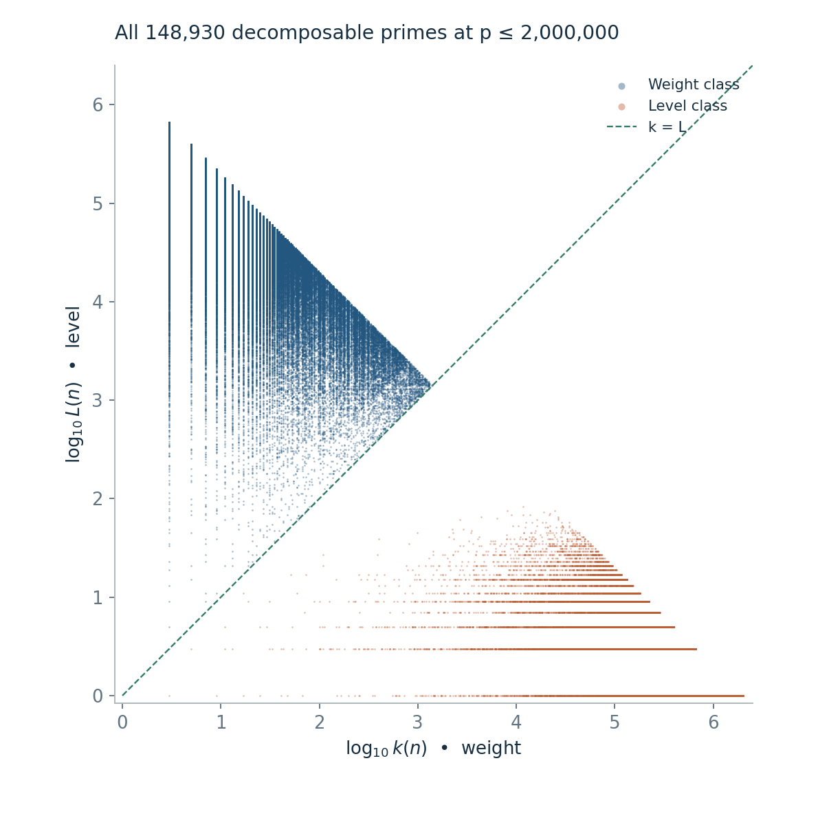
Blue denotes the weight class, including ties; copper denotes the level class. Newly generated weight–level plots use square canvases, identical axis ranges, and equal aspect. All mathematics, figures, data, and interaction needed to read this file are embedded; an internet connection is needed only to follow source links.
Significance
1.1 The construction’s mathematical content
The distinctive object is a local pair . The jump first reflects the successor across the current term, producing . The same jump then supplies the lower threshold in a divisor search. Thus additive information does two jobs: it determines the integer to be factored and the part of its divisor spectrum that is eligible.
The identity alone would allow many decompositions. The rule selecting the smallest divisor greater than the jump makes the coordinates canonical. This rule is where the framework becomes a definite mathematical object. Its uniqueness is a consequence of minimisation in a finite ordered set, while its arithmetic behaviour depends on the factors of the reflected integer.
There are three distinct grounds for studying it. First, it offers an exact dictionary: least prime factors in the natural-number base case, twin primes in one prime-weight column, and congruence-conditioned gaps in other columns. Second, its classification creates a divisor-window counting problem with a natural geometric boundary. Third, its atlas makes the same construction available across many sequences, enabling comparisons once their cutoffs, growth rates, and arithmetic constraints are controlled.
1.2 What the coordinates add
A coordinate transformation can be useful without supplying additional information. For a decomposable term, the complete triple determines both members of the original pair:
Conversely, the original pair determines the triple. The transformation reorganises existing information so that particular events become simple regions, columns, or lines. The useful question is whether that reorganisation produces a proof, a sharper estimate, or a reliable new statistic.
The classification alone is much coarser. It discards the numerical coordinates and retains only which side of contains the point. Its rarefaction can therefore conceal differences in the composition of the two classes. The same total proportion can arise from different populations of level-one terms, composite weights, or residue locks.
1.3 Native questions and inherited difficulties
The level-classified count is a natural question generated by this construction. Saying that the weight-3 column is infinite, however, says precisely that there are infinitely many twin primes. These are different kinds of mathematical yield. An exact reformulation is useful for navigation, but establishing the equivalence supplies no lower bound for the original prime family.
Nor is an attractive cloud of points itself an independence or randomness test. The observed large-scale shape has a substantial deterministic component, and related rarefaction appears in random controls. A persuasive contribution must identify what remains after those geometric and statistical effects have been accounted for.
Definitions, existence, and geometry
2.1 The exact definition
Let be a strictly increasing sequence of positive integers. For each term whose successor is known, define
When , it is itself an eligible divisor; the minimum exists. The decomposition then holds with and . When , those zeros are a sentinel for failure: they do not assert the identity .
A term is decomposable if and only if , and its triple is then unique.
Indeed, is equivalent to , hence . Once this holds, the least member of the nonempty finite divisor set is unique, and division determines . The strict inequality matters at the boundary.
A finite list therefore needs one extra term to classify its last requested entry. For a prime-value cutoff , the successor of the last prime at most must still be generated, even when it exceeds .
2.2 Euclidean division and its boundary
On the decomposable domain, the definition is equivalent to selecting the least admissible modulus satisfying
The residue class alone does not express minimality. The exact search set is . On arbitrary pairs, one must retain the decomposition gate: when , every modulus gives remainder but quotient zero. Such a pair is not decomposable in WLJ. The supplied modular report usefully distinguishes this general-sequence boundary from the OEIS definition on consecutive primes. [5,6]
2.3 Classification as an empty divisor window
A decomposable term is level-classified when , and weight-classified when . Ties belong to the weight class. For a positive integer , write for its positive divisors.
Since , the first equivalence follows by multiplying by . The second follows because is the first divisor beyond . Including the upper endpoint in the window assigns to the weight class.
Also, on the level class, and . Minimality forces . This elementary observation explains why the level branch of the plots remains low.
Two consecutive prime pairs already illustrate the mechanism:
Both have . The threshold 2 selects divisor 3; the threshold 4 skips it and selects 5. The class changes even though the reflected integer and its factorisation are identical.
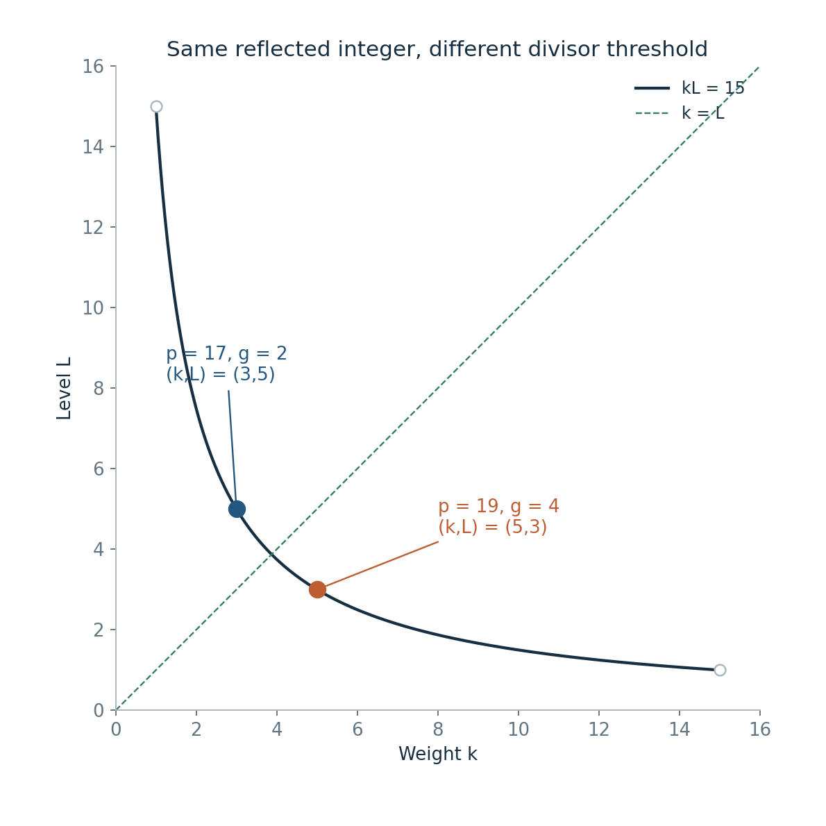
2.4 What is intrinsic and what depends on the sequence
The triple belongs to the pair, not to the isolated integer. In the natural sequence, gives ; in the prime sequence, gives . Rescaling or translating a sequence also changes the divisor search and need not transport the weights by the same rescaling or translation.
The existence criterion gives a simple growth classification. If , every sufficiently large term is decomposable. This applies to increasing polynomial sequences of positive degree. If the ratio is eventually at least , no sufficiently large term is decomposable. At the boundary, the strict inequality must be tested term by term. These are existence results, not distribution laws for weights or levels.
The fundamental theorem of arithmetic and Eratosthenes
3.1 The natural-number base case
For , the gap is 1. Thus, for ,
where is the smallest prime factor. The least divisor greater than 1 must be prime: if it were composite, one of its proper factors would be a smaller divisor greater than 1.
In the natural-number sequence, is level-classified if and only if is prime. Equivalently, the level class is exactly the shifted primes, and every member has .
If is prime, . If is composite, its smallest prime factor satisfies ; therefore . This includes prime squares on the diagonal.
The shift is essential: the classified integer is , whereas primality is being tested for . The line should be labelled “shifted primes” when the dataset is the sequence of natural numbers.
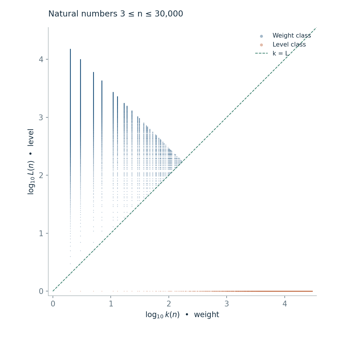
3.2 Why the sieve picture is exact
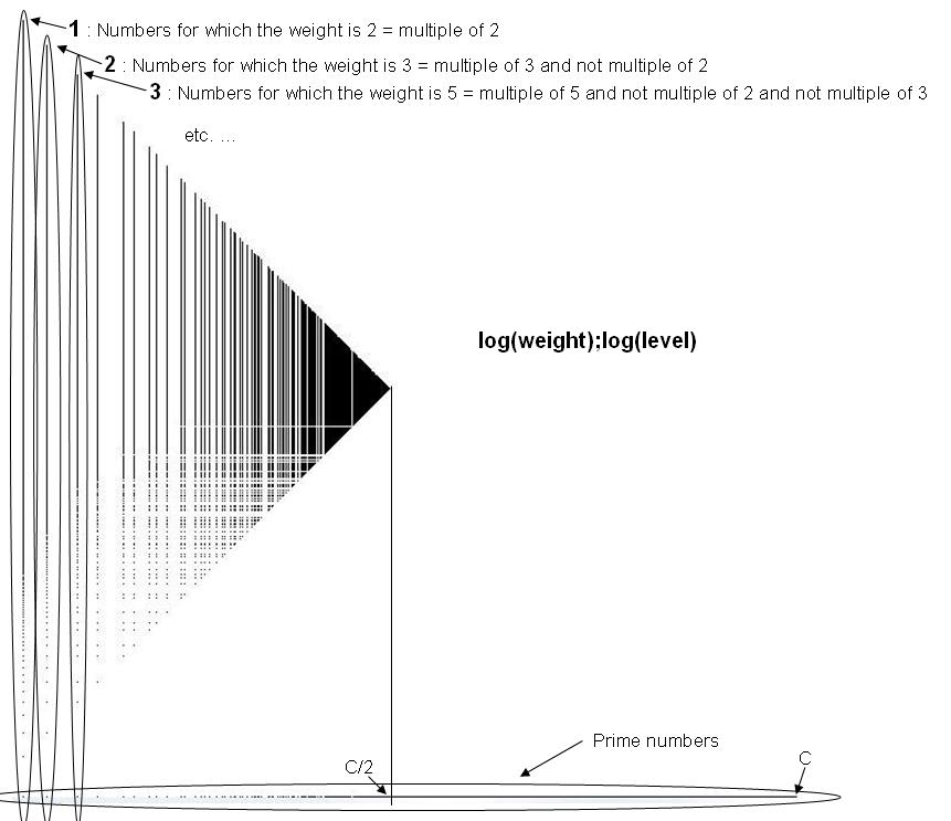
Assign each composite integer to the first prime that divides it. The column contains even ; the column contains multiples of 3 not already assigned to 2; and each later prime column contains the multiples first reached at that sieve stage. The prime itself appears at , while the composite part of its column begins at .
This is the partition underlying the sieve of Eratosthenes, expressed through least prime factors. WLJ generalises the classification rule by replacing threshold 1 with a sequence-dependent gap. It does not automatically generalise the computational performance of a sieve that marks many multiples in one pass. For a prime sequence, the successor prime is already an input to the decomposition.
3.3 The relation with the FTA
The fundamental theorem of arithmetic guarantees a unique prime factorisation of . That factorisation determines its divisor set and provides an efficient route to finding the weight. But a WLJ weight can be composite, because its smaller prime factors may all lie below the gap. The prime , with and , has weight 9.
One WLJ triple records a selected factor and its cofactor; it is not generally the full prime factorisation. In the natural case, repeated smallest-prime-factor extraction recovers that full factorisation. To implement this through the original sequence definition, a cofactor is processed as the natural-number pair , whose reflected integer is . Applying the natural decomposition to itself would instead factor .
Selection uniqueness and unique factorisation should therefore remain separate ideas. The former follows from the ordered divisor search. The latter is a theorem about multiplication in the integers. Their interaction is useful; neither should be used as an unproved slogan for the other.
3.4 A precise connection with the prime number theorem
Among decomposable natural terms at most , the level fraction is exactly
The asymptotic follows directly from the prime number theorem. It explains rarefaction in the base-case picture. Applying the classifier to the prime sequence asks a different question, with a different population and a variable gap. The analogy motivates the question but does not prove the corresponding density statement.
Prime numbers: structure, proofs, and conjectures
4.1 Notation and a verified starting table
For consecutive primes and , write . On the decomposable domain, . The main sequence identifiers are:
| Quantity | Meaning | OEIS |
|---|---|---|
| Prime sequence | A000040 | |
| Consecutive prime gap | A001223 | |
| Reflected integer, or zero | A118534 | |
| Weight | A117078 | |
| Level | A117563 |
The weight and level entries were checked against their current OEIS pages. The first 17 primes below were recomputed and checked against the founding paper’s Table 2. [1,5]
| n | p(n) | p(n+1) | g | l | k | L | Class |
|---|---|---|---|---|---|---|---|
| 1 | 2 | 3 | 1 | 0 | 0 | 0 | Unclassified |
| 2 | 3 | 5 | 2 | 0 | 0 | 0 | Unclassified |
| 3 | 5 | 7 | 2 | 3 | 3 | 1 | Level |
| 4 | 7 | 11 | 4 | 0 | 0 | 0 | Unclassified |
| 5 | 11 | 13 | 2 | 9 | 3 | 3 | Weight · tie |
| 6 | 13 | 17 | 4 | 9 | 9 | 1 | Level |
| 7 | 17 | 19 | 2 | 15 | 3 | 5 | Weight |
| 8 | 19 | 23 | 4 | 15 | 5 | 3 | Level |
| 9 | 23 | 29 | 6 | 17 | 17 | 1 | Level |
| 10 | 29 | 31 | 2 | 27 | 3 | 9 | Weight |
| 11 | 31 | 37 | 6 | 25 | 25 | 1 | Level |
| 12 | 37 | 41 | 4 | 33 | 11 | 3 | Level |
| 13 | 41 | 43 | 2 | 39 | 3 | 13 | Weight |
| 14 | 43 | 47 | 4 | 39 | 13 | 3 | Level |
| 15 | 47 | 53 | 6 | 41 | 41 | 1 | Level |
| 16 | 53 | 59 | 6 | 47 | 47 | 1 | Level |
| 17 | 59 | 61 | 2 | 57 | 3 | 19 | Weight |
The only non-decomposable primes are .
Nagura’s theorem gives a prime between and for ; hence a prime has successor less than . The primes below 25 are checked directly. In particular, is decomposable, while is not. [7]
4.2 Parity, coprimality, and divisor localisation
For a decomposable prime, is odd and is even. Consequently are odd. Also , so
Every divisor of , including and , is therefore coprime to the gap. Since a level-classified term has , parity sharpens the general bound to
For the weight class, . Thus its gaps automatically satisfy a square-root upper bound. Rarefaction of the complementary class would still allow infinitely many exceptional large gaps; a density-zero statement does not give a pointwise bound for every prime.
4.3 Twin primes and the mod-3 rigidity
For primes , if and only if are twin primes.
If , the even positive gap is less than 3, hence equals 2. Conversely, for a twin pair above 3, neither nor is divisible by 3. Therefore is divisible by 3, and 3 is the smallest divisor of exceeding the gap 2.
If , then . If , requiring both and to avoid zero modulo 3 forces , giving . Since is even, and are equivalent.
The founding paper’s Conjectures 7 and 8 are an implication and its contrapositive; they are not two independent conjectures. The current OEIS project page marks them as elementary. The biconditional above also records the complementary case. [6]
4.4 A sharp cubic bound, with its correct scope
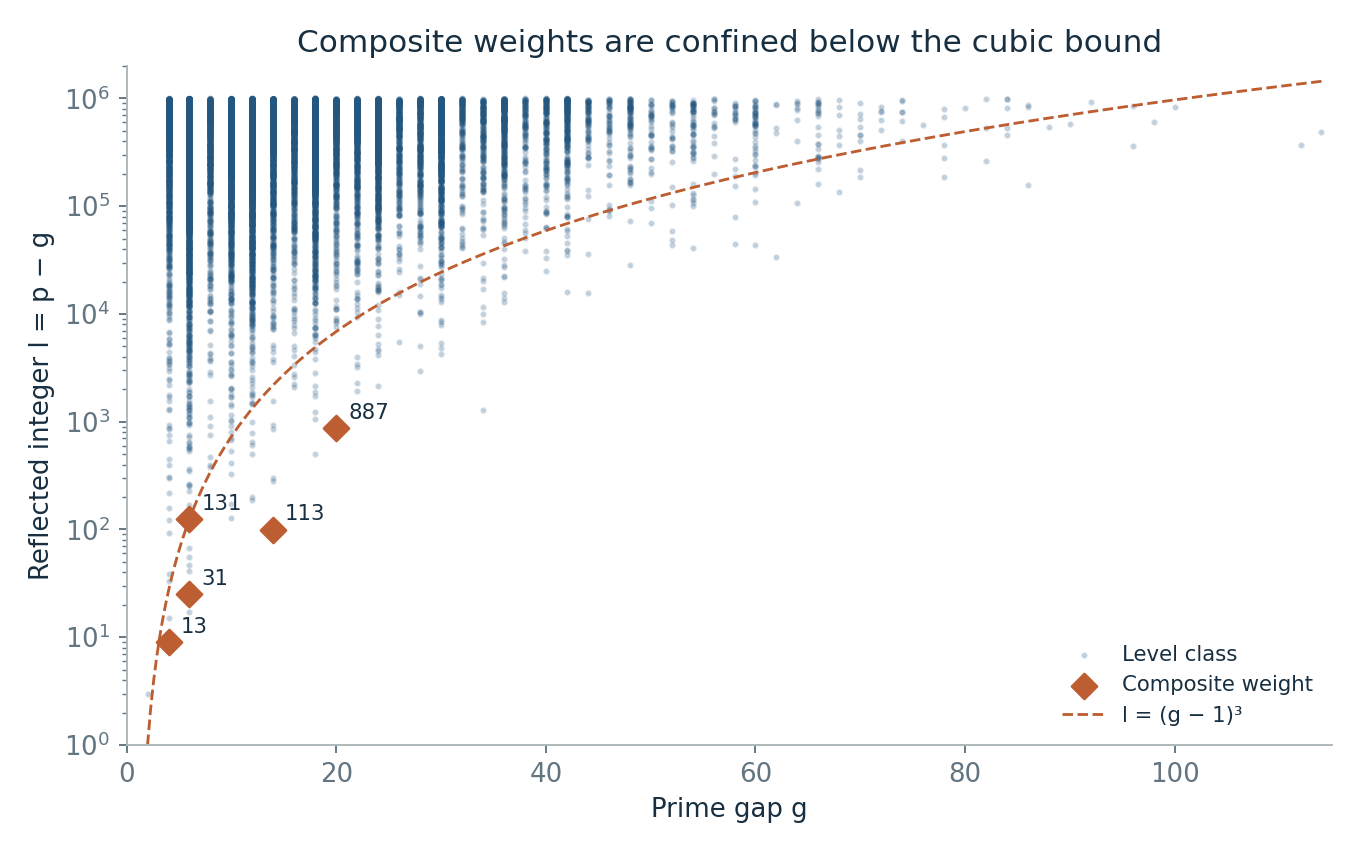
If a prime is level-classified and its weight is composite, then
Write with . Both and divide , so minimality of implies . They are odd; hence . Together with , this gives . Equality is attained at , where and .
Our complete run through finds precisely the following composite-weight level-classified primes:
| p | g | l | k | L |
|---|---|---|---|---|
| 13 | 4 | 9 | 9 | 1 |
| 31 | 6 | 25 | 25 | 1 |
| 113 | 14 | 99 | 33 | 3 |
| 131 | 6 | 125 | 25 | 5 |
| 887 | 20 | 867 | 51 | 17 |
The later project reports give a finite extension of this list to , using exhaustive prime-gap tables. This report carries that historical statement with its bound; it does not revalidate the full external gap database. A universal cubic inequality and a list closed below a finite height are distinct from the founding paper’s Conjecture 4, which asserts the list is complete for all primes. The latter does not follow solely from those two results. [2–4]
4.5 Level one and reflected prime triples
A level-one term has , meaning that has no proper divisor exceeding . If is prime, this is automatic. Conversely, when , a composite has a proper divisor , where . Thus
The unqualified equivalence is false: and have but composite reflected integers 9 and 25. The fresh census finds no additional such examples through . For all , the safe counting identity is
where counts decomposable primes at most with prime, and counts the level-one terms with composite . The historical finite closure gives for . It does not justify replacing by 2 for unrestricted .
A prime counted by lies in the arithmetic progression , and the last two primes must be consecutive. If also , then is balanced: its two adjacent gaps are equal. All balanced primes lie in this level-one subclass; the converse requires that additional predecessor condition. Infinitude of the balanced subclass would imply infinitude of the level class. Infinitude of the larger class would not establish infinitude of the balanced subclass.
4.6 The rarefaction theorem and its proof architecture
Write , counting only decomposable primes. The current ledger records the following unconditional result with an internal-review asterisk:
This is the project’s resolution of the founding rarefaction conjecture. The account below explains the reduction and the analytic input; it is not an external referee report. [2–4]
Let . For gaps , telescoping gives for sufficiently large , and therefore at most such primes. This controls the large-gap tail without an upper bound on every individual gap.
For , place the terms with in a small exceptional box. In fact , so the number of distinct primes in this box is ; the looser bound used in the reports also suffices. This step absorbs composite weights without assuming that their global exception list is finite.
Every remaining level-classified term has prime weight , odd , and, writing , three prime linear forms:
An upper bound may count all such triples, dropping the requirement that the latter two primes be consecutive. This enlarges the set in the permitted direction. The proof then needs an upper-bound Selberg sieve for these three forms, uniform for the polylogarithmic parameters . Local obstructions, primes dividing coefficients, and small exceptional solutions must be included in that uniform statement. General sieve background is available in Tao’s exposition. [10]
The project bounds the local singular factors by an absolute multiple of , with . The elementary mean-value estimates and lead to
The chosen yields the stated result. The -sum accounts for the logarithmic factor. The standard sieve input is the analytic part that deserves an explicit, independently checked uniform formulation. The divisor reduction and the gap-tail bound are transparent and do not depend on the finite census.
Three limits should remain clear. Density zero is compatible with an infinite or a finite level class. The theorem does not assert that every successive finite proportion decreases. Finally, fitting a decreasing diagnostic such as cannot verify the asymptotic upper bound or its implied constant.
4.7 Why twice the twin-prime constant appears
There is an exact arithmetic calculation behind the proposed level-one constant. For the progression pattern , define
The product vanishes unless : otherwise the pattern covers every residue modulo 2 or 3. When ,
To average over gaps, write the last multiplicative factor as , supported on squarefree integers with prime factors at least 5 and . Since converges, expanding the divisor sum and averaging multiples of gives
The exact local identity
then reduces the mean to , where is the twin-prime constant. The factor at 3 is ; it converts into . This identity and average are unconditional. The fresh truncated products and elementary tail bounds certify the displayed approximation . [2,3]
A sufficient modelling formulation is that the counts of prime triples with the upper pair consecutive are jointly approximated by
with errors summable to , negligible gap tails at that same scale, and . Under these explicit joint assumptions, summing the progression series with the exponential weight gives the proposed asymptotic. The constant is fixed exactly; the validity of the model and its limiting error are separate issues. A finite percent-level residual neither proves nor disproves eventual asymptotic agreement.
4.8 The census and the conjecture ledger
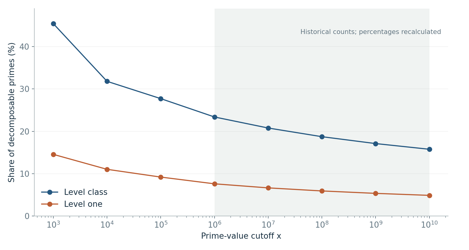
The following table uses prime values , not the first primes. This matters when comparing it with the founding paper’s tables indexed by the number of primes. Percentages have been recalculated from the integer counts.
| Cutoff x | Decomposable | Level class | Level one | Ties | Level share | Counts |
|---|---|---|---|---|---|---|
| 1,000 | 165 | 75 | 24 | 3 | 45.4545% | Fresh |
| 10,000 | 1,226 | 390 | 135 | 6 | 31.8108% | Fresh |
| 100,000 | 9,589 | 2,658 | 880 | 8 | 27.7193% | Fresh |
| 1,000,000 | 78,495 | 18,353 | 5,953 | 12 | 23.3811% | Fresh |
| 2,000,000 | 148,930 | 33,454 | 10,851 | 14 | 22.4629% | Fresh |
| 10,000,000 | 664,576 | 138,049 | 44,011 | 28 | 20.7725% | Carried |
| 100,000,000 | 5,761,452 | 1,078,707 | 339,870 | 79 | 18.7228% | Carried |
| 1,000,000,000 | 50,847,531 | 8,692,339 | 2,708,031 | 187 | 17.0949% | Carried |
| 10,000,000,000 | 455,052,508 | 71,670,808 | 22,083,608 | — | 15.7500% | Carried |
| Item | Statement | Status and scope |
|---|---|---|
| C1 | Infinitely many weight-3 primes | Equivalent to twin primes; open. |
| C2 | Every odd weight k ≥ 3 occurs infinitely often | Open fixed-column prime-pattern family. |
| C3 | Every odd level L ≥ 1 occurs infinitely often | Open; retain the distinction between all terms at a level and level classification. |
| C4 | Only five level-classified primes have composite weight | Cubic bound proved; exception list closed over stated finite ranges. The unrestricted original claim does not follow from the finite closure. |
| C5 | Infinitely many level-(1;1) primes | Balanced-prime infinitude; open. |
| C6 | Infinitely many level-(1;i) primes for every i ≥ 1 | Open predecessor-index family; requires primality of the reflected integer. |
| C7–C8 | The mod-3 implications | Proved elementary background; one implication and its contrapositive. |
| C9 | Level-classified primes have relative density zero | Theorem 1 in the current project; internally audited, not externally refereed. |
| Level-one law | N₁(x) ∼ 2C₂ x / log²x | Conditional model; joint consecutiveness assumptions must be stated. |
| Native infinitude | Is the level class infinite? | Open in the examined ledger; stronger subclass conjectures would suffice but are not equivalent. |
“Polignac-type” is a description of the fixed-gap and prime-pattern difficulties in these families. It should not be promoted into a literal equivalence with one standard conjecture without proving both implications for the particular column or line.
Analysis of the supplied graphs
5.1 The geometry before the pixels
In ordinary coordinates, each decomposable term is on its own hyperbola . Put , , using the same logarithm base on both axes. Then
Thus a fixed reflected integer becomes a line of slope , and the classification boundary is . On an equal-aspect plot, the signed perpendicular distance from the diagonal is . It measures a logarithmic factor ratio. Stretching one axis changes that geometric meaning.
For a cutoff , the roof is already imposed by . On the weight side, . These two inequalities explain much of the triangular upper-left boundary. For primes, the lower-right level lines also satisfy . A finite plotted maximum gap therefore produces a low level sheet; it is not an asymptotic limit on levels.
5.2 The two natural-number images
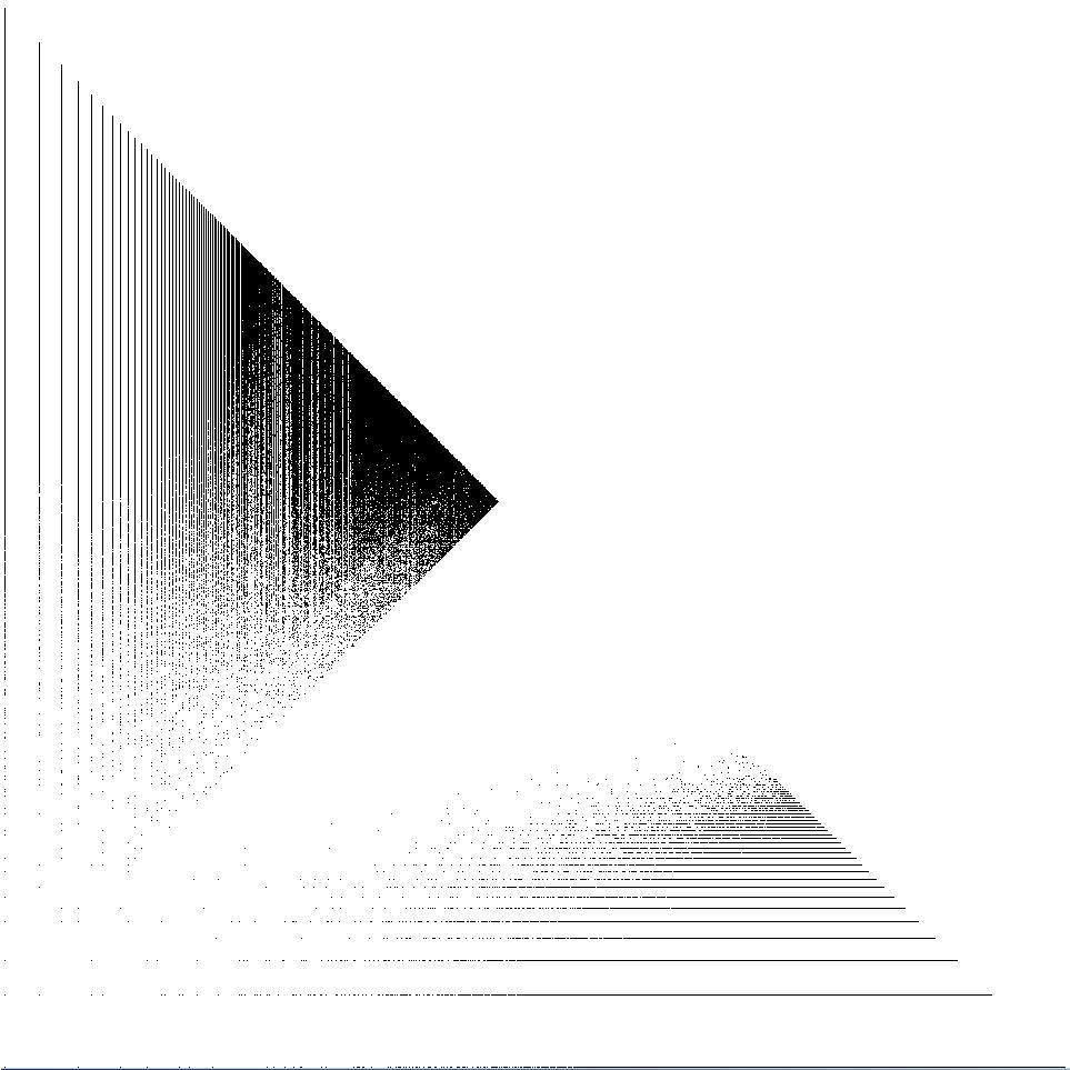
sieveNb.jpg. The annotated columns correctly describe the first-prime-divisor partition when “multiple of 2”, “multiple of 3”, and similar labels refer to . The lower line consists of shifted prime inputs. The tip occurs near half the logarithmic range because prime squares have , while the outer prime baseline extends to .
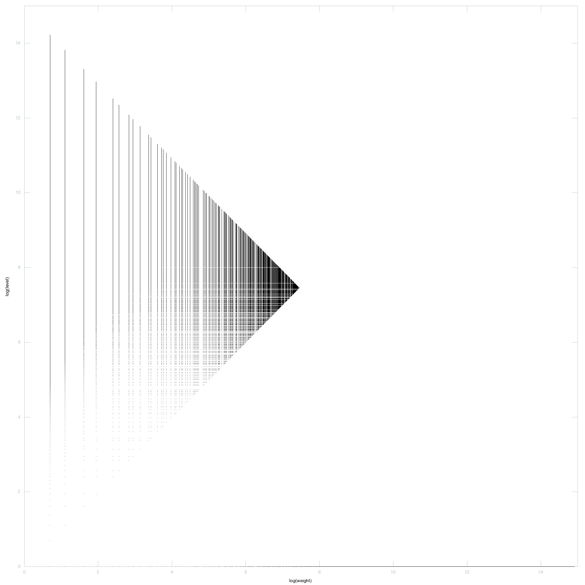
naturaldecomp3M-2048.jpg. The high-resolution image exposes the same column structure over a larger range. Its filename suggests a three-million-term scale, but the raster alone does not certify the generating dataset. Dense dark regions indicate overplotting as well as occupancy. Darkness cannot be converted into an exact count without the underlying rows and rendering settings.
5.3 The annotated prime map and the large two-wing plot
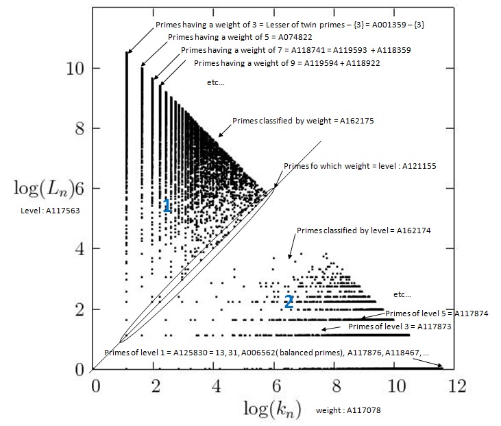
classification_primes.jpg. Its upper-left striations are constant-weight columns; the lower-right striations are constant-level lines. The weight-3 identification with lesser twin primes is exact, with 3 excluded. The diagonal consists of ties and belongs to the weight class. Square reflected integers do not all give ties: the selected divisor must itself equal their square root.
Log_L-Log_k_1500000-R.jpg. The two wings are a useful overview of the divisor-window split. The tall leftmost prime column is . The sparse-looking lower structure contains discrete odd levels, including the full baseline. Its filename and earlier descriptions suggest a sample indexed by 1.5 million primes; no raw dataset accompanying this image was available to verify the precise cutoff. No class percentage is inferred from its area or darkness.
The fresh Figure 5 reproduces the structural features at a completely specified value cutoff. Its 22.46% level share also illustrates why a percentage from one historical cutoff should not be reused as the caption for another. The eighth edition’s Figure 2 count and percentage are corrected in the current treatise and in this report’s audit.
5.4 The two 3D screenshots
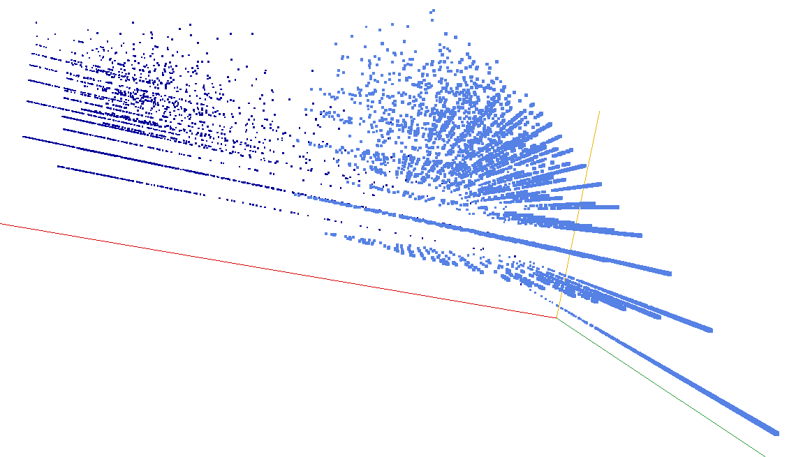
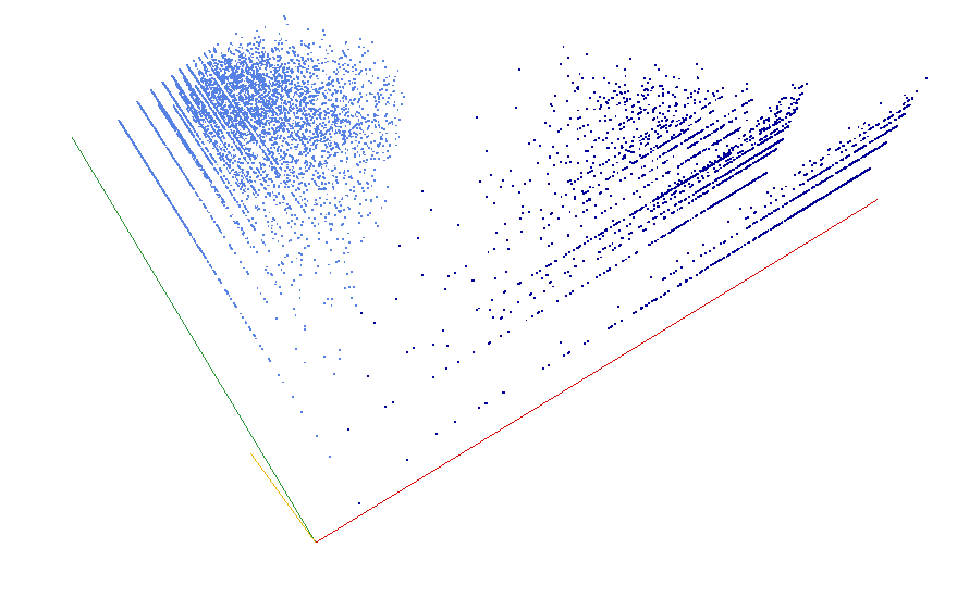
The two supplied 2018 screenshots show different viewpoints of the prime construction in logarithmic weight, level, and jump coordinates. The current linked 3D page confirms this axis convention. Its current advertised sample is a property of that page, not proof of the historical screenshots’ exact datasets. [8]
With , fixed-gap layers satisfy , while fixed reflected integers satisfy . The horizontal projection recovers the 2D classification plane. The third coordinate can separate points that overlap in 2D and can display how rows change with gaps.
Perspective views distort apparent slopes and distances and hide points behind other points. The screenshots are therefore best used to identify strata and choose slices for further measurement. They do not establish a fractal dimension, independence between coordinates, or an additional invariant from visual appearance alone. Camera settings, axis scaling, and a downloadable point table should accompany any quantitative use.
5.5 The status-ledger screenshot
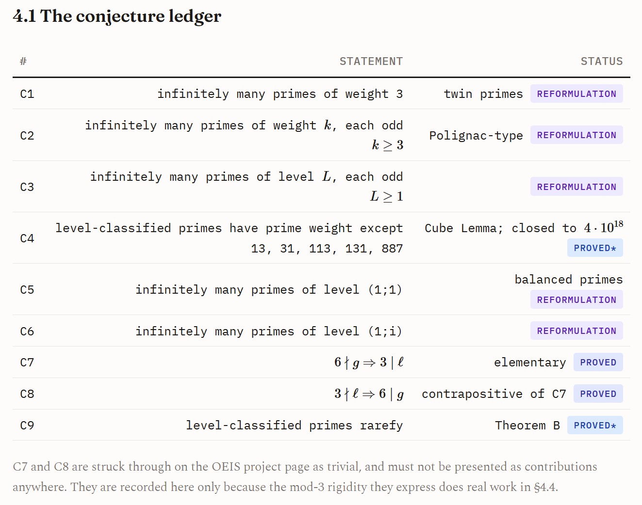
Capture d’écran 2026-07-29 125239.jpg is documentary evidence of an earlier ledger, not a numerical graph. It records the project’s evolution, including the elementary status of the mod-3 implications and the rarefaction proof asterisk. The current written ledger and precise theorem statements take precedence. In particular, a finite closure height cannot be dropped when summarising the listed composite-weight exceptions.
5.6 What measurements reveal beyond the overall wings
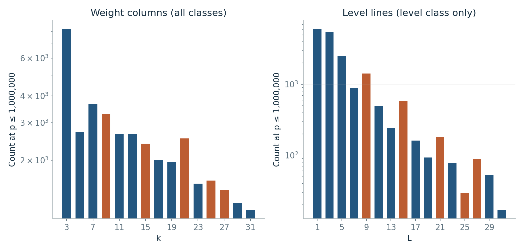
The column profile is visibly non-monotone: a larger weight can occur more often than a smaller one. This is expected once columns are understood as unions of admissible gap and residue events. The level profile also has arithmetic structure; a feature such as the prominence of levels divisible by 3 must be interpreted together with the exact mod-3 relation and the gap distribution.
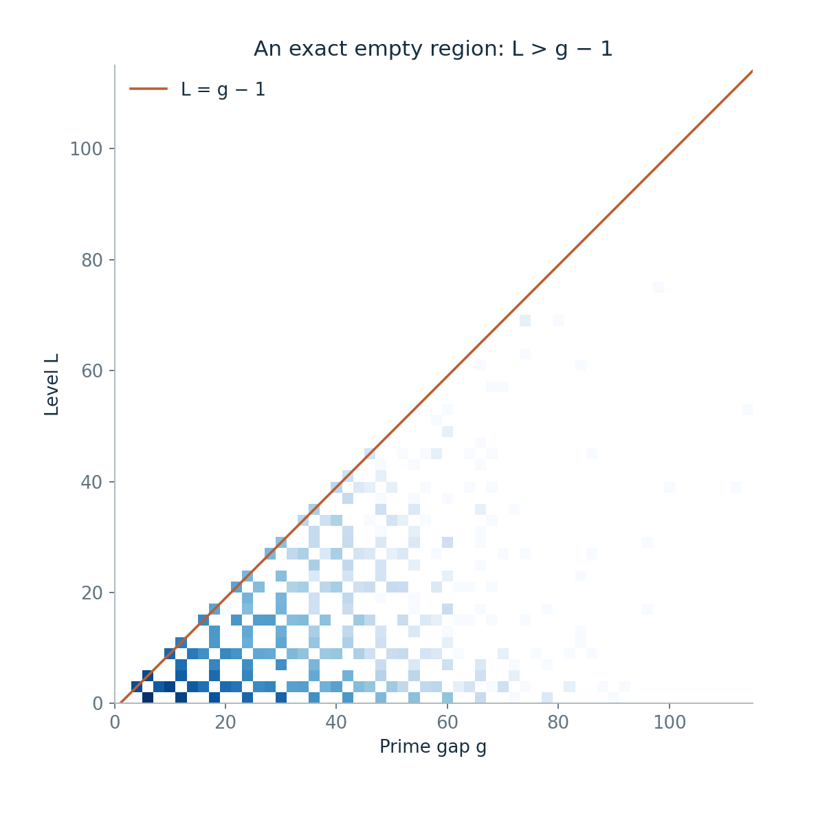
5.7 An inspectable prime atlas
The panel below uses precomputed, verified rows for every decomposable prime at most . Change the gap or class filter; hover over a point to read its exact pair and decomposition. The axes stay fixed and equal. Filtering changes the population, not the coordinate system.
Hover over a point to inspect its exact decomposition.
5.8 Random controls: similar shape, different composition
The supplied eighth-edition census compared primes with an independent Cramér sequence, selecting each integer with probability about , and an odd-integer model with probability about on odd candidates. It reports close aggregate tracking for its classic-model run and a higher level share in the odd model. That is evidence about those experiments, rather than a theorem covering every sequence of the same density. [2]
We ran three fresh seeds per model through the general integer classifier at . Both models use probabilities capped at 1 near the origin. A generated successor beyond the cutoff is retained. Their results are:
| Population | Sampling | Level share | Level-one share |
|---|---|---|---|
| Primes | Exact census | 23.3811% | 7.5839% |
| Cramér: all integers | 3 fresh seeds | 23.8587% range 23.8171–23.8923% | 7.9338% range 7.8248–8.1254% |
| Cramér: odd integers | 3 fresh seeds | 28.8865% range 28.7810–28.9730% | 15.8094% range 15.6048–15.9480% |
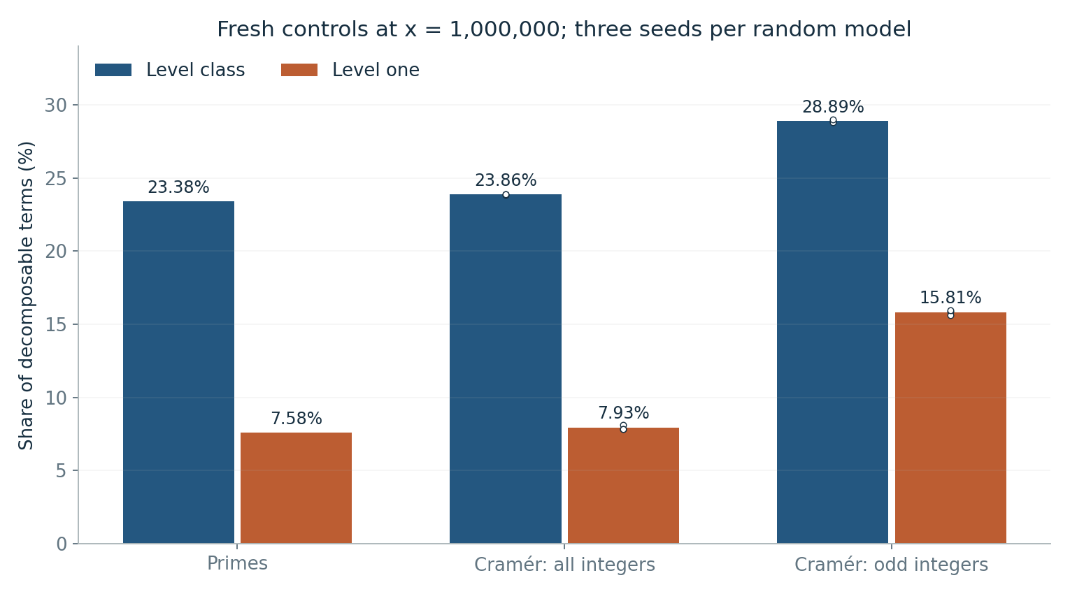
The classic model again has a comparable level share, but these seeds do not reproduce a literal 1% relative agreement with the primes. The odd model substantially changes the level-one proportion despite its similar overall density and prime-like parity. This gives a concrete reason to compare conditional arithmetic statistics, not only the total class fraction.
Possible impacts at the additive–multiplicative interface
6.1 An exact bridge: columns as gap-and-residue events
For any positive modulus , divisibility of the reflected integer gives the exact relation
For a fixed proposed weight , one additionally excludes every divisor in . This converts a multiplicative event into a finite combination of residue tests conditioned on the additive gap. It is an exact bridge, although counting its prime solutions remains difficult.
The gap is even and smaller than the weight. Gap 2 already forces weight 3. At gap 4, the only possible smaller eligible divisor before 7 is 5, since is odd. At gap 6, no integer lies strictly between the gap and 7. These observations prove both directions. The fresh prime census checks both identities with zero violations.
This translation is more informative than saying that the framework “combines addition and multiplication”. It specifies exactly which residue events make up particular weight columns and supplies independent ways to check a census.
6.2 A local null model and its missing conditioning
Fix a prime modulus and consider prime endpoints larger than . Their residues exclude and . The lock residue is one of the remaining classes. A uniform endpoint-residue model therefore assigns it mass .
Consecutiveness imposes more conditions: each interior even offset , , must be composite. A residue can force one such point to be composite whenever that point exceeds . Such a class has one fewer interior primality event to suppress. This changes its weight among consecutive prime pairs.
The eighth edition develops a first-order “interior-credit” model and fits a further multiplier. Its useful contribution is a mechanism that can be tested by residue-resolved counts. The fit is not an exact local probability law, and a coefficient estimated on a given collection of cells requires testing on new ranges and cells before it is treated as transferable. In particular, empirical agreement at gaps 2 and 4 is not exact equidistribution of finite residue counts.
6.3 The connection with divisors in intervals
Ford’s theory studies integers having divisors in specified intervals; Koukoulopoulos treats related questions for shifted primes. WLJ’s level event is precisely a missing-divisor condition, so this literature is directly relevant. The obstacle is that both the shifted integer and the divisor interval depend on the actual next-prime gap. A theorem for a fixed shift cannot simply be substituted with that random-looking, arithmetically dependent shift. [11,12]
A successful transfer would require a uniform estimate in the shift and interval parameters, with an error that survives averaging over consecutive gaps. Establishing that estimate would produce a substantive theorem at the interface: existing multiplicative machinery would control an event defined by the local additive ordering of primes.
6.4 A neighbouring analytic programme
Gafni and Tao study rough numbers inside consecutive prime gaps. They obtain an upper bound of order for their exceptional-gap count and a conditional asymptotic under a prime-tuples hypothesis. Their object differs from WLJ’s reflected integer outside the gap, but the use of sieve bounds and singular-series averages offers a concrete methodological comparison. Their theorem does not itself prove a WLJ estimate. [13]
6.5 What the atlas could contribute
The project website provides a large sequence atlas with 2D views, 3D views, and downloadable data. It also explicitly cautions that its data have not all been verified. The atlas becomes a stronger research instrument when each sequence carries a reproducible definition, cutoff convention, successor policy, exact arithmetic audit, and appropriate control. [8]
A useful comparative descriptor would include decomposability, level share, level-one share, occupied weights, ties, and residue-conditioned deviations. The comparison should distinguish fixed-value cutoffs from fixed-rank cutoffs. A polynomial sequence and a prime-like random sequence should not be compared solely at the same number of terms and then interpreted as having the same density.
6.6 Generalisations: opportunities with prerequisites
Polynomial sequences already offer a concrete laboratory without changing the ambient integers. For squares , and ; decomposition begins at . This links the divisor search to values of a quadratic polynomial. For triangular numbers, decomposition likewise begins at , with . These statements follow by direct substitution and were checked computationally.
Moving to is more delicate. Polynomial rings have subtraction and divisibility, but no intrinsic analogue of the positive-integer order used by “next”, “greater than the gap”, and “smallest”. A degree-and-lexicographic order adds choices, and existing irreducible-tuple results do not automatically control consecutiveness in that order. A useful analogue must first specify its order, unit convention, nonzero domain, and a substitute for the inequality .
The same caution applies to algebraic integers and monoids. One can often choose a divisor canonically after adding an order, but that alone does not recover the original Euclidean-remainder interpretation. The research target should be a precise analogue with proved properties, rather than a shared notation.
6.7 Conditions for a larger mathematical impact
| Possible impact | Concrete achievement required |
|---|---|
| Pedagogical | A reliable visual dictionary linking prime gaps, divisor windows, and residue restrictions. |
| Experimental | Statistics that distinguish arithmetic sequences from carefully matched controls on fresh data. |
| Analytic | Uniform counting estimates for moving shifts and divisor thresholds, with controlled consecutive-gap errors. |
| Algorithmic | A proved or reproducible improvement over relevant algorithms, counting factorisation and successor-generation costs. |
| Structural | An extension whose central statements are independent of arbitrary choices, or whose dependence on those choices is characterised. |
These are plausible directions, with different burdens of proof. The material examined supplies no deduction concerning the Riemann hypothesis and no new solution of Goldbach or the twin-prime conjecture. Any such connection would need an additional, explicit mathematical implication. The native results and open problems are sufficient grounds for evaluating the construction on its own terms.
Detailed conclusion and future research
7.1 Conclusions supported by the analysis
WLJ turns a local successor relation into a canonical divisor problem. The construction is exact wherever it is defined, has a simple existence criterion, and recovers the least-prime-factor partition on the natural numbers. Its weight–level geometry is therefore mathematically interpretable: the diagonal is a divisor-window boundary, the upper roof is a product cutoff, and much of the visible striation is the discreteness of fixed factors and cofactors.
On the primes, the framework has a coherent elementary theory. Parity, coprimality, the twin column, mod-3 rigidity, level localisation, and the composite-weight cubic bound all have short proofs. The explicit column identities add a useful dictionary between divisibility and gap-conditioned residues. These statements survive changes in sampling range and do not rely on the appearance of a plot.
The rarefaction proof has a meaningful native architecture: isolate large gaps, force prime weights outside a small box, and apply a uniform sieve to three linear forms. The project’s internal theorem status should remain visible until that analytic input and its implementation receive independent review. Submitting a manuscript does not by itself constitute external verification.
The exact singular-series mean explains why enters the level-one model. It does not alone prove a counting asymptotic. The additional condition that two of the three primes be consecutive must be treated as part of the joint model, not assumed to disappear because a marginal gap distribution is available.
The computations support the established small census and the geometric analysis. They also illustrate the need for explicit provenance: the exceptional set is ; the two-million plot has a level share of 22.46%; and new random seeds need not reproduce an earlier percentage tolerance. Such corrections sharpen the research object without changing its definition.
7.2 A prioritised research project
| Priority | Question and deliverable | What would count as progress? |
|---|---|---|
| 1 · Proof audit | Write Theorem 1 as a separate manuscript with a precise uniform sieve lemma, parameter ranges, and local exceptional cases. | An independent check of every implication and summed error; the finite exception census is not used as a global theorem. |
| 2 · Joint level-one model | State the additional conditional hypothesis behind the reflected-prime/consecutive-gap intersection. Analyse the interior constraints at the same asymptotic scale as the main term. | A justified derivation of the constant and an error term, or a rigorously identified correction to the proposed asymptotic. |
| 3 · Lock residuals | Fit a residue-resolved consecutiveness model on one range; test it on new ranges, moduli, and gaps. | Accurate predictions beyond the fitting sample and a principled account of correlated cells and finite-size errors. |
| 4 · The level-above-one count | Seek the order of , with , using divisor-interval methods. | A uniform estimate that handles the moving shift. A candidate constant must remain stable under window and normalisation changes. |
| 5 · Infinitude | Investigate whether the level class is infinite; distinguish the whole class from each fixed level and the balanced-prime subclass. | An unconditional construction or lower bound. A density-zero upper bound is compatible with either answer. |
| 6 · Certified atlas | Attach a compact certificate to each sequence: input definition, cutoff, successor, kernel, checksum, and matched controls. | Reproducible deviations beyond density and congruence baselines, followed by targeted proofs or conjectures. |
| 7 · Other ambient rings | Define one polynomial-ring analogue completely before undertaking a large census. | An existence/uniqueness theorem, a meaningful base case, and an explicit account of dependence on the chosen order. |
7.3 A practical experiment on the lock mechanism
A focused next experiment would record, for every selected gap and prime modulus , the full histogram of . It would retain both all prime endpoint pairs of separation and the subset that are consecutive. Comparing those two populations isolates the effect that the current heuristic is trying to explain.
The first model is uniform over endpoint-admissible residues. The second incorporates which interior offsets are forced composite. A third adds pairwise interactions between interior offsets. These models should be compared on withheld prime-value windows, without refitting their coefficients there. This distinguishes a mechanism that transfers from a descriptive fit to one census.
The relevant failure conditions are informative: systematic residuals tied to particular interior patterns, coefficients drifting with the cutoff, or good aggregate predictions with poor residue predictions. Each failure would indicate which part of the joint conditioning still needs arithmetic input.
7.4 The appropriate standard for the framework
The strongest outcome would be a reusable theory of divisors evaluated at shifts selected by a sequence’s own gaps. A narrower successful outcome would be a well-audited collection of exact identities, a native density theorem, and experimental methods that detect where simple models fail. Both are concrete mathematical objectives.
The framework should be judged by the results and questions it makes precise: what is proved, what becomes calculable, and what new estimate remains to be established. Its geometric language is valuable when it makes those distinctions easier to see.
Numerical audit, corrections, and reference code
A.1 What was computed for this report
The prime census was freshly generated through , with a successor beyond the cutoff. A sieve of smallest prime factors supplied exact divisors of each positive ; the least divisor above the gap gave , and integer division gave . A separately written divisor-pair scan agreed on every one of the 78,498 prime pairs with current prime at most , including the three non-decomposable cases.
The 17 initial rows were matched to the paper’s table and the live OEIS sequence beginnings. Exact reconstruction, coprimality, parity, mod-3 rigidity, the twin column, both small-column identities, the level bound, and the composite-weight cubic bound were checked over all 148,930 decomposable rows. All checks passed. The control experiments deliberately used the general-sequence classifier, rather than a prime-specific parity shortcut.
This is a targeted extension of the recorded audit, not a new claim to have rerun the historical or census. The higher-cutoff rows are carried from the supplied eighth edition. Their percentages were recomputed, while the underlying high-range counts were not independently regenerated here.
Random controls used NumPy’s PCG64 generator with seeds 20260905, 20260906, and 20260907. For each seed, independent uniforms were drawn for integers 3 through 1,000,200, first for the classic model and then for the odd model. Only current terms at most 1,000,000 were counted. The exact output summary is embedded below for download; these three runs are a reproducible finite experiment, not an uncertainty estimate for all possible controls.
A.2 Source corrections retained or identified
| Issue | Treatment in this report |
|---|---|
| Project-context exception list | Use , established directly and confirmed by the sources. The prime 5 is decomposable. |
| Eighth-edition Figure 2 | At , use 148,930 points and a 22.4629% level share. The printed 148,932 and 16.9% are not used. |
| Original Conjecture 4 | Separate the universal cubic inequality from the five-element list verified to a finite height. Sharpness at 131 does not require a global uniqueness claim for equality. |
| Level-one counting identity | Use for unrestricted ; replace by 2 only inside a stated verified range. |
| Conditional Theorem 2 | Make the joint consecutiveness assumption explicit. Marginal H1 and H2 alone do not justify the decoupling step. |
| Earlier proposed growth law | The expression , printed as a proposed order for in the seventh and eighth editions, exceeds the scale of . It cannot be correct. A share of order would correspond to a count of order ; that conversion does not prove either law. |
| Constant and per-gap fit | Use the exact corrected Euler product for , not the old misprinted digits. The eighth edition’s correction to its earlier per-gap tolerance is retained; no uniform tolerance is inferred from a plot. |
| Tuple ordering in algos.txt | Several routines return on failure but on success. Use the consistent sentinel from the supplied fordiv kernel. |
A.3 Constants: verification at the precision used
With prime factors included through , the fresh products are and . These are truncated products, not the infinite constants. Bounding the remaining prime sum by the corresponding integer sum gives
For the first inequality use on the tail. For the second, expanding bounds it by for . These intentionally conservative bounds certify the four-decimal values and after rounding. Higher precision quoted in the earlier reports was not re-certified here.
A.4 The supplied PARI/GP reference kernel
The following is the attached decompwlj_fordiv.txt kernel, reformatted without changing its rule. Its input contract is positive integers . For integer arguments, the PARI documentation specifies increasing divisor order in fordiv, which is essential to returning the minimum. [9]
decomp(a,b) =
{
  my(d=b-a,l);
  if(a<=2*d, return([0,0,d]));
  l=a-d;
  fordiv(l,k, if(k>d, return([k,l/k,d])))
}

\\ 0: unclassified; 1: weight (including ties); 2: level.
dclass(r) = if(!r[1],0,if(r[1]>r[2],2,1));

\\ Input validation can be applied without changing the kernel.
decomp_checked(a,b) =
{
  if(type(a)!="t_INT" || type(b)!="t_INT" || a<1 || b<=a,
     error("need positive integers a < b"));
  decomp(a,b)
}

\\ Representative checks: [weight, level, jump].
decomp_checked(5,7)      \\ [3,1,2]
decomp_checked(7,11)     \\ [0,0,4]
decomp_checked(11,13)    \\ [3,3,2] : tie, weight class
decomp_checked(13,17)    \\ [9,1,4]
decomp_checked(72,76)    \\ [17,4,4] : general bound L=d
decomp_checked(131,137)  \\ [25,5,6] : cubic equality
PARI/GP was not installed in this report’s execution environment, so no new PARI run is claimed. The decomposition kernel is reused from the supplied source; its displayed numerical outputs were checked independently by exact integer computation. The project’s prior PARI version and cross-checks remain historical provenance.
The divisor stage examines at most divisors after factorisation; that does not make total running time . The cost of factoring , ordering/enumerating divisors, arithmetic on large integers, and generating the successor must be included. A trial-division implementation also needs careful accounting when the descending level branch starts at a large gap. No algorithmic speedup over established prime generation or factorisation is claimed here.
Sources and provenance
Web sources were consulted on 5 September 2026. File sources were read directly from the supplied copies. Mathematical arguments marked “proved” in the report are written out; carried data and source-reported proof status are identified separately. References to the current treatise concern its status ledger and scope checks; the detailed historical discussion also draws on the supplied editions.
- Rémi Eismann. Decomposition into weight × level + jump and application to a new classification of primes, arXiv:0711.0865v4, 18 January 2010. Supplied PDF inspected, including its 17-prime table and original conjecture wording. Read together with the later corrections.
- Supplied project report. Fable5_decompwlj_deep_analysis_8th_edition_final_2026_08_07.html, 7 August 2026. Definitions, census, singular-series calculation, column identities, controls, and corrections. Public copy.
- Supplied project report. Fable5_decompwlj_deep_analysis_7th_edition_2026_08_05.html, 5 August 2026. Proof architecture, original-conjecture mapping, and prior computational provenance. Public copy.
- Current project reference. A Pedagogical Treatise, Ninth Edition, 16 August 2026. Located online and inspected, especially §§3–5, §8 ledger, §9 algorithms, and Appendix A. It supersedes earlier editions on current project status; qualifications in this analysis preserve the distinction between a finite verification and an unrestricted theorem.
- OEIS. Current entries A117078 and A117563, checked for the definitions and initial terms. Supplied GPTSol_decompwlj_modular_arithmetic_report_2026-08-06.html also read for the general-sequence remainder boundary.
- OEIS project exposition. Decomposition into weight × level + jump. Current public definitions, sequence dictionary, algorithms, and historical conjecture labels. The living project ledger is used where its status is more recent.
- Jitsuro Nagura. On the Interval Containing at Least One Prime Number, Proceedings of the Japan Academy 28 (1952), 177–181. DOI: 10.3792/pja/1195570997.
- Rémi Eismann’s atlas. decompwlj.com and the prime 3D graph. The supplied links.txt guided these source checks. All seven supplied images are reproduced with their historical status intact.
- PARI/GP documentation. Programming in GP: control statements, entry
fordiv. The supplied algos.txt and decompwlj_fordiv.txt were inspected directly. - Terence Tao. The prime tuples conjecture, sieve theory, and the work of Goldston–Pintz–Yıldırım, Motohashi–Pintz, and Zhang (2013). Primary exposition of prime-pattern upper bounds and the distinction between sieve upper bounds and prime-tuple asymptotics. The project proof cites Halberstam–Richert’s Sieve Methods; that book’s exact theorem numbering was not independently checked here.
- Kevin Ford. The distribution of integers with a divisor in a given interval, Annals of Mathematics 168 (2008), 367–433. Primary reference for divisor-interval counting.
- Dimitris Koukoulopoulos. Divisors of shifted primes, arXiv:0905.0163; International Mathematics Research Notices 2010, 4585–4627. Primary reference for the fixed-shift comparison; it is not cited as a ready-made WLJ theorem.
- Ayla Gafni and Terence Tao. Rough numbers between consecutive primes, arXiv:2508.06463 (2025). A related but distinct consecutive-gap problem.
This report is a new synthesis and audit. It does not silently update the supplied source documents or assign itself a new edition number in their series.